RealValue House Prediction
A UTMIST project by Arsh Kadakia, Sean Wu, Matthew Leung, Alex Liu, Charles Ding, Sepehr Hosseini
RealValue is a machine learning project for predicting home prices in Toronto. Using TensorFlow convolutional neural networks in conjunction with a dense network component, owners can take a couple of pictures of their home, enter a few simple details, and receive an accurate price range of what their home is worth. This ease of use allows homeowners to be confident about their residential decisions and be more informed about the real estate market than ever before.
Motivation and Goal
In Toronto, residential sales have grown by a figure of 35.2% year-over-year from January 2020 to January 2021. As COVID-19 slows down and consumers look to get back to spending, this trend shows no signs of slowing down.
Furthermore, this new trend provides an incredible opportunity for home owners who would like to take advantage of the “hot” market. However, finding what your home is worth is a very tricky process that may involve fully committing to specific realtors, or having to remodel your home for “selling purposes” that may not be comfortable to a home-owner. As a result, many home-owners will lose out on the opportunity of a lifetime.
RealValue provides a solution to this problem by allowing homeowners to understand their home’s worth from the comfort of their phone.
By only providing pictures of the house and some primary house numbers such as number of bedrooms, bathrooms and square footage, the goal is to create an algorithm that can predict a house’s price in the range of 20%. For example, for a house truly worth 500,000, a predictive range of 400k-600k is quite informative and marks the point of success for this project.
Dataset
California Dataset
We initially trained our network on a dataset of California houses, created by Ahmed and Moustafa, consisting of both structured data (statistical property information in tabular form) and unstructured data (images). This dataset contains information for over 500 houses, each with 4 images of a bathroom, bedroom, kitchen, and frontal view. Statistical information for each house includes the number of bedrooms, bathrooms, square footage, postal code, and price.
Toronto Dataset
The main goal of our project was to create our own network for Toronto houses. Hence, we created our own Toronto real estate dataset by compiling the images, prices, number of rooms, surface areas, and postal codes of houses on the Toronto Regional Real Estate Board (TRREB) website. A Python script was used to accurately calculate the area of the house from provided measurements of each room. Like the California dataset, in our Toronto dataset, we had 4 images for each house for the frontal view, bedroom, bathroom, and kitchen.
Cleaning / Feature Engineering
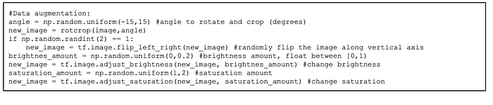
We first performed data augmentation on the raw images by passing them through a series of transformations including random angle rotation (±15 degrees), cropping, flipping, brightness changes, and saturation changes. One augmented image was produced for every raw image, doubling the total number of images.

Next, we produced a one-to-one mapping between image data and price label by combining the 4 images (frontal, bedroom, bathroom, kitchen) for each house into a single image. Images were combined to a single mosaic, in a 2x2 fashion, where each quadrant consisted of one of the 4 images.
For the statistical data, the number of bedrooms, bathrooms, square footage and price were normalized using min-max normalization. However, the Zip Code attribute brought together an interesting idea. There are 2 ways to encode location information. The first is to simply one-hot encode zip codes and train the network that way. The other way is to get the latitude and longitude of a given zip code and normalize those coordinates. In our training infrastructure, we allowed for both types of encoding to see which one performs better.
Network Structure
In this problem of real estate price prediction, we needed a network architecture that would accept multi-inputs and mixed-data, namely images and numerical data. Thus, we created a network consisting of two branches: a CNN for input images, and a dense network for input statistical data (e.g. price, number of rooms, square feet). The image of the house that was merged was fed into the CNN, while corresponding numerical data for that house was fed into the dense network. Then, at the end, the results from both branches were concatenated together and then passed through one fully-connected layer (a logistic regression unit). Finally, a single value is outputted, which is the price of the house.
We employed a configuration file that controlled the various hyperparameters of our prediction model. Examples of user-controllable choices include a choice of the CNN model, choice of the dense model’s layer sizes, choice of the optimizer, learning rate, etc.
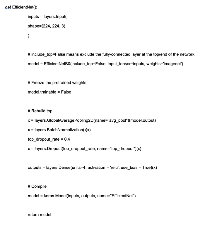
The CNN model that yielded the best results for us was an EfficientNetB0 architecture that contained pre-trained weights from ImageNet. We also tried ResNet, RegNet, LeNet, and VGG16.
We configured the model by replacing the original top layers with a custom top that consisted of a pooling, batch normalization, dropout, and dense layer. This allowed us to employ EfficientNet as a feature extractor which we used to extract features from our own images.
Training
Our network was first trained on a dataset for California houses. We split our dataset into 80% training, 5% validation, and 15% test. All of the features in the California dataset were used. The CNN, dense network and logistic regression unit were all trained at the same time.
After trial and error, we found the best hyperparameters to be:
- Optimizer: Adam
- Momentum: 0.1
- Weight Decay: 0.1
- Learning Rate: 0.001
- Number of Epochs: 100
These hyperparameters ended up being the same for zip code training and continuous latitude and longitude training. The results for latitude and longitude training will be discussed in the following section.
For the Toronto dataset, we split our dataset into 90% training, 2.5% validation and 7.5% test. The test dataset size had to be decreased slightly due to the low number of training examples.
In terms of one-hot encoding, implementing transfer learning was not possible due to differences in the number of zip codes between the California and Toronto datasets.
Transfer Learning
After training our network on the California dataset, we saved the weights of the network, then applied transfer learning to a dataset of Toronto houses which we collected.
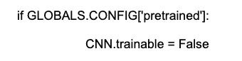
The weights in the CNN were reused from the California dataset by disabling weight updates as below. This choice was made as the nature of the images did not change in any way.
The dense network weights were not reused during transfer learning. This is because the normalized latitude and longitude values for the Toronto dataset were completely different inputs in comparison to the original California dataset.
Results
Altogether, using an EfficientNet pretrained model with only the fully-connected layers changed, we received a 21% error on the California dataset trained by one-hot encoding zip codes.
For latitude and longitude training, on the California dataset however, the error was significantly higher, with test error being 33%. This appears slightly problematic initially, as the latitude and longitude training process is used for transfer learning later.
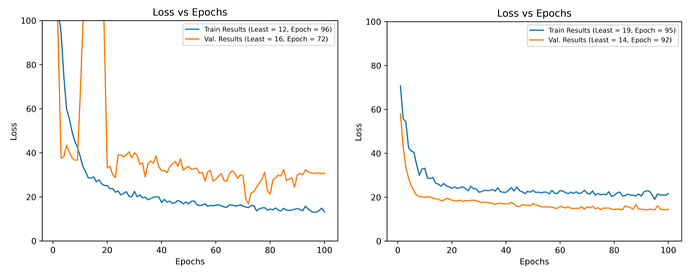
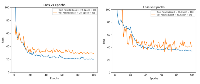
However, the same did not hold true for the Toronto dataset. While both zip code training and transfer learning generated strong sub-20% error results, transfer learning demonstrated a noticeably cleaner training curve, thereby indicating greater stability.
Furthermore, the test error for the transfer learning portion (with latitude and longitude instead of zip codes) was 14.9%, almost 2% lower than the 16.9% test error on the zip code training version of the Toronto dataset.
Altogether, it can be concluded that transfer learning had a positive effect on the overall training process, increasing accuracy and adding training stability.
Conclusion
The goal of this project was to create a high-accuracy CNN and dense network that can take in image inputs and text inputs to provide a strong estimate for house prices. In this aim, our group succeeded by creating a sub-15% loss model for the Toronto dataset of houses.
Furthermore, this model has succeeded as a proof-of-concept idea. House images can be taken into consideration in order to provide a highly accurate price estimate. Given significantly more data, it is therefore reasonable to assume that the model may go below 10% loss. We have also created a training infrastructure that allows for the inclusion of more training data without any overhead costs.
If you would like to take a look at the code for our project, please take a look at our GitHub repository here.
Furthermore, if you would like to try our algorithm on your own house (with some limitations), head on over to https://myrealvalue.ca.